A Quantitative Approach to Personalized Investment Planning

Most investment advice boils down to vague principles: "diversify," "think long-term," "don't panic." That's fine as far as it goes, but it doesn't help you answer the questions that actually matter: How much do I need to save each month to retire comfortably? What mix of assets gives me the best return for the risk I'm willing to take? How likely am I to actually reach my financial goals?

These are quantitative questions, and they deserve quantitative answers. In this post, I walk through the mathematical frameworks behind investment planning - from compound interest and Monte Carlo simulations to Modern Portfolio Theory and rebalancing. The examples use Indian Rupees, but the concepts apply universally. The goal is to give you the tools to make investment decisions based on data and math, not gut feeling.

Disclaimer: I am not a SEBI-registered investment advisor, and nothing in this post constitutes personal financial advice. What I'm sharing here are the quantitative techniques I use for my own investment planning. Treat this as learning material, not a recommendation - always do your own research or consult a qualified advisor before making financial decisions.

The Power of Compound Interest

Everything in investment planning starts with one idea: money grows over time. A rupee invested today is worth more than a rupee invested next year, because this year's returns generate their own returns next year. This is compound interest, and understanding the math behind it is the foundation for everything that follows.

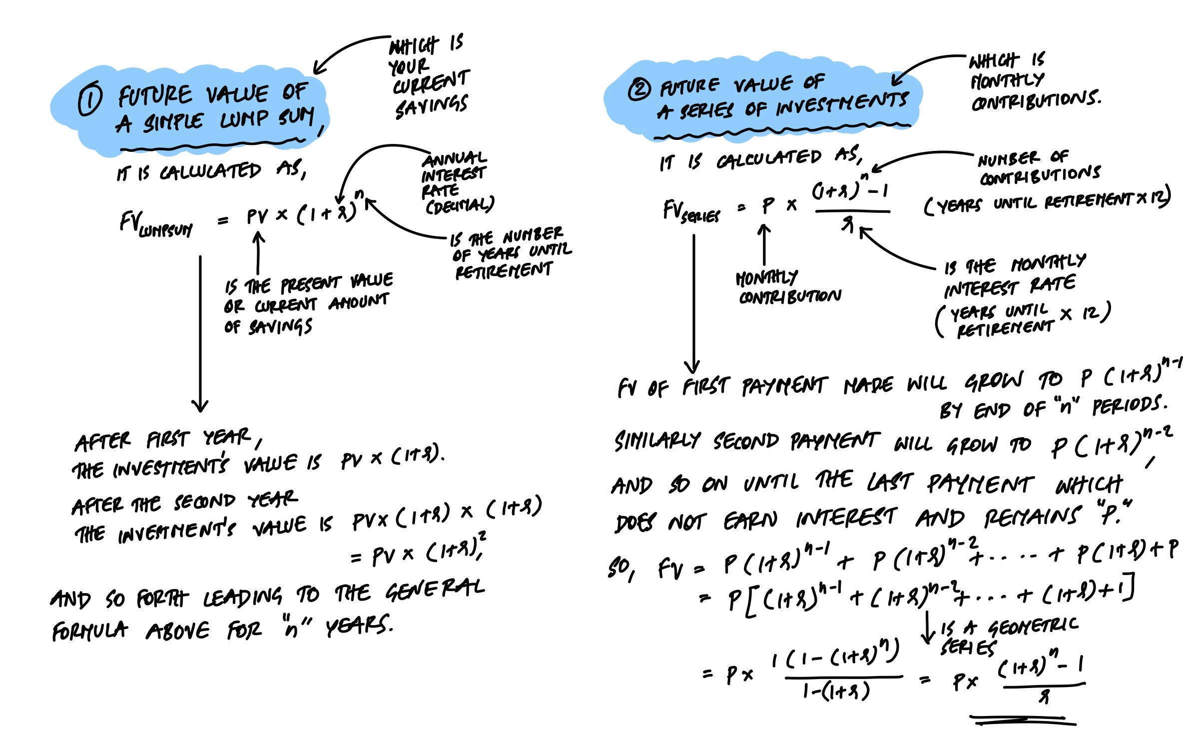
The future value of an investment has two components. The first is the growth of money you already have (a lump sum). The second is the growth of money you add regularly over time (a series of contributions). The formulas are shown below.

A Retirement Example

Say you're planning for retirement 25 years from now. You currently have ₹500,000 in savings, and you plan to contribute ₹10,000 per month. Assuming an average annual return of 7% (a realistic figure for a diversified portfolio in India), what will your retirement fund look like?

• The future value of your current ₹500,000, compounded annually at 7% over 25 years: approximately ₹27,13,716.
• The future value of your monthly contributions of ₹10,000 at the same rate over 25 years: approximately ₹81,00,717.
• Combined, your retirement fund would be approximately ₹1,08,14,433 (₹1.08 crore).

This illustrates something important: the monthly contributions account for roughly 75% of the final value, even though the lump sum had a 25-year head start. Regular, disciplined investing matters more than the size of your starting amount.

Lump Sum vs. Regular Contributions

In practice, you should use a combination of both. A lump sum investment generally performs better in markets that trend upward over the long term, because the entire amount has more time to compound. But regular contributions (SIP - Systematic Investment Plan) provide a benefit called dollar-cost averaging: when markets dip, your fixed contribution buys more units at lower prices, which can smooth out volatility over time.

Modeling Uncertainty: Monte Carlo Simulations

The retirement example above assumes a constant 7% return every year. But real markets don't work that way. Some years you get 15%, other years you lose 8%. The question isn't just "what's the expected outcome?" - it's "what's the range of possible outcomes, and how likely am I to reach my goal?"

This is where Monte Carlo simulations come in. The idea is simple: instead of assuming one fixed rate of return, you simulate thousands of possible scenarios, each with randomly sampled returns drawn from a probability distribution based on historical data. Each simulation gives you one possible path your investment could take. Run 1,000 of them, and you get a picture of the full range of outcomes - from best case to worst case and everything in between.

How It Works

1. Define the distribution. Based on historical data, set the expected return (mean) and volatility (standard deviation) for each year. For our example: 7% mean, 3% standard deviation.
2. Sample randomly. For each year of the investment horizon, draw a random return from that distribution.
3. Compute the path. Apply each year's sampled return to the portfolio, adding the annual contribution.
4. Repeat. Do this 1,000 times to generate 1,000 different possible outcomes.
5. Analyze. Look at the distribution of final values to understand the probability of reaching your target.

The Simulation

Using the same parameters as our retirement example (₹500,000 initial investment, ₹120,000 annual contribution, 25-year horizon, 7% expected return, 3% standard deviation), here are 1,000 simulated paths:

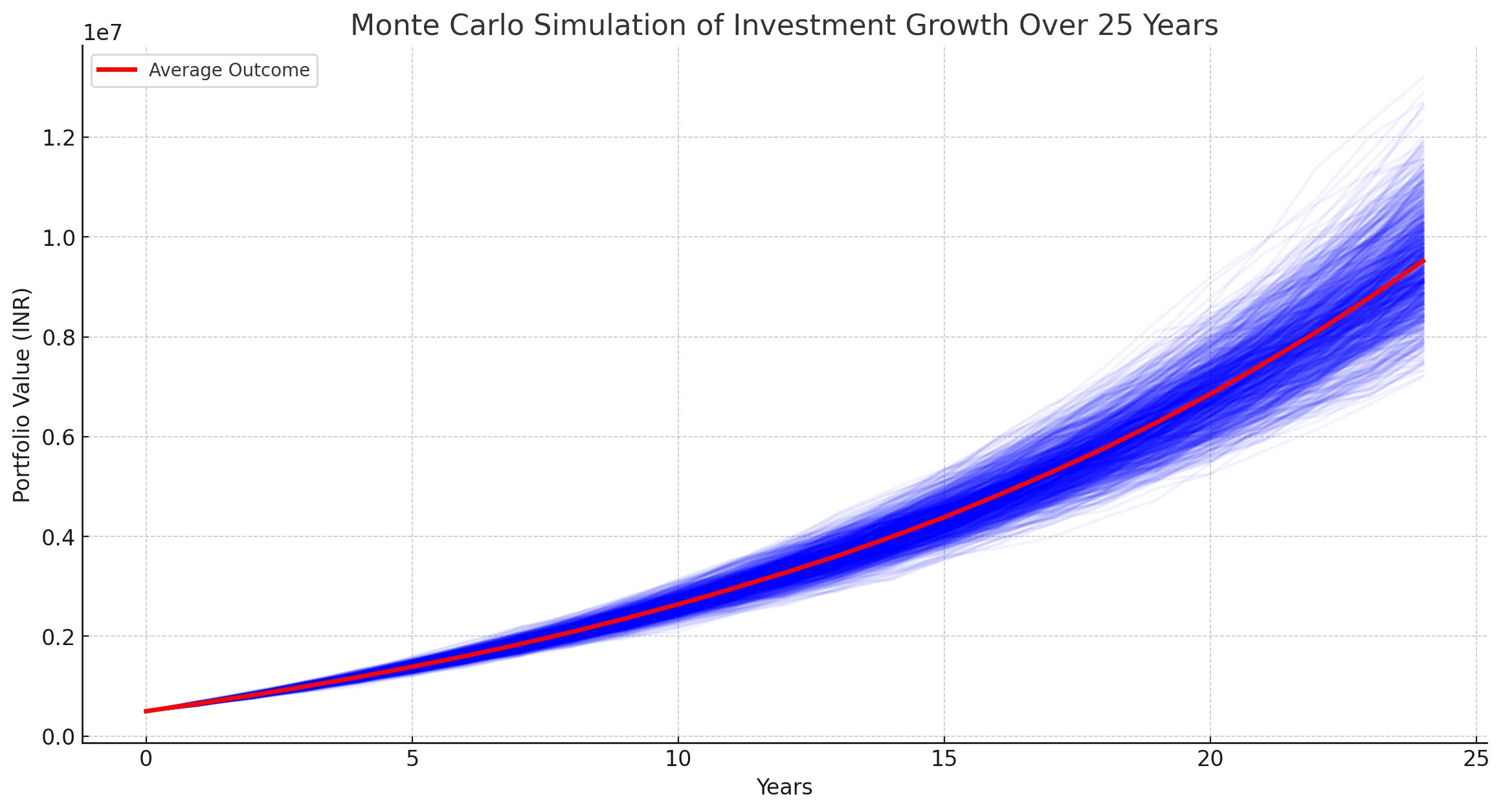
Each blue line is one possible future. The red line is the average across all 1,000 simulations. Notice the fan shape - the uncertainty grows with time. In the early years, the paths are tightly clustered. By year 25, the spread between the best and worst outcomes is enormous.

This is the real value of Monte Carlo simulations: they turn a single number ("you'll have ₹1.08 crore") into a range of probabilities. You can ask: "What's the probability I'll have at least ₹80 lakhs?" or "What's the worst case in the bottom 10% of scenarios?" That's much more useful for actual planning than a single point estimate.

Understanding Your Risk Profile

Before deciding how to invest, you need to understand how much risk you're comfortable with. Risk tolerance isn't just about how much volatility you can handle emotionally - it depends on your goals, your timeline, your income needs, and your experience.

Risk Assessment

A simple risk questionnaire scores you on five dimensions. For each, choose the option that best matches your situation:

1. Investment Goal and Time Horizon
   A. Capital preservation, under 2 years (Score: 1)
   B. Moderate growth, 3-5 years (Score: 2)
   C. Growth-focused, 6+ years (Score: 3)
2. Experience with Investments
   A. None (Score: 1)
   B. Limited - mostly fixed deposits, bonds (Score: 2)
   C. Experienced - stocks, mutual funds, other securities (Score: 3)
3. Reaction to Market Downturns
   A. Sell to minimize losses (Score: 1)
   B. Hold and wait for recovery (Score: 2)
   C. See it as a buying opportunity (Score: 3)
4. Expected Rate of Return
   A. Up to 5% per annum, very low risk (Score: 1)
   B. 5-10% per annum, moderate risk (Score: 2)
   C. 10%+ per annum, willing to accept high volatility (Score: 3)
5. Income Requirement
   A. Need current income from investments (Score: 1)
   B. Some income preferred, but not essential (Score: 2)
   C. No income needed - prefer reinvesting for growth (Score: 3)

Scoring:

• 5-8 points: Low risk tolerance. Conservative investments - fixed deposits, bonds, stable value funds.
• 9-12 points: Moderate risk tolerance. Balanced mix - hybrid funds, mix of equities and fixed income.
• 13-15 points: High risk tolerance. Growth focused - diversified equity portfolios, high-growth mutual funds, ETFs.

Visualizing Portfolio Volatility

Once you know your risk profile, you can simulate what a portfolio at that risk level actually looks like over time. Consider a moderate-risk portfolio: 60% equities (average return 10%, standard deviation 15%) and 40% bonds (average return 5%, standard deviation 5%). Running 1,000 simulations over 20 years:

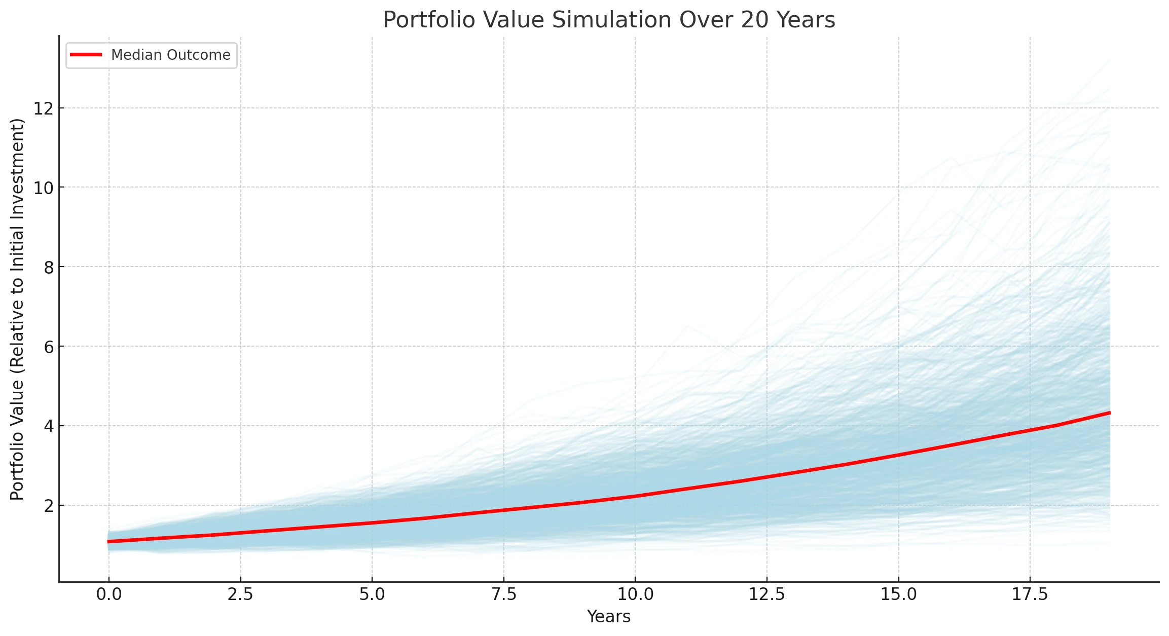
The red line here shows the median outcome rather than the average. Why median instead of average? Because investment returns can produce extreme outliers - a few incredibly lucky scenarios would skew the average upward, making the "typical" outcome look better than it actually is. The median gives you a more honest picture of what a typical investor would experience.

The spread of paths shows the trade-off clearly: equities introduce volatility (the wide fan of possible outcomes), while bonds provide stability. The combination smooths things out, but doesn't eliminate uncertainty. This is why understanding your risk tolerance matters - you need to be comfortable with the range of outcomes your portfolio can produce, not just the expected one.

Building the Portfolio: Modern Portfolio Theory

Now we get to the central question: given a set of available assets, how do you find the best combination? This is the problem that Harry Markowitz solved in 1952 with Modern Portfolio Theory (MPT). The key insight is that the risk of a portfolio depends not just on the risk of individual assets, but on how those assets move in relation to each other.

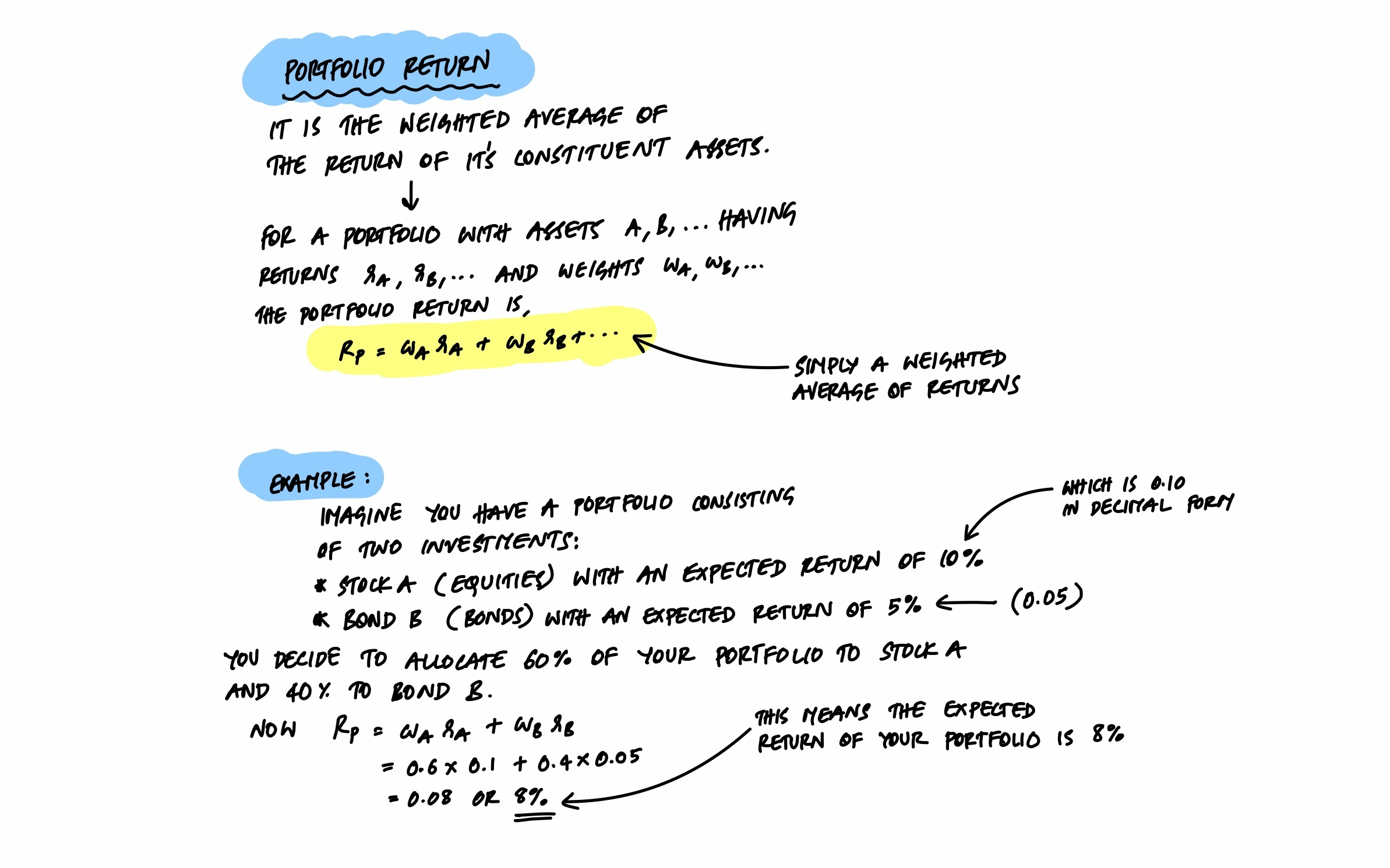
Portfolio Return

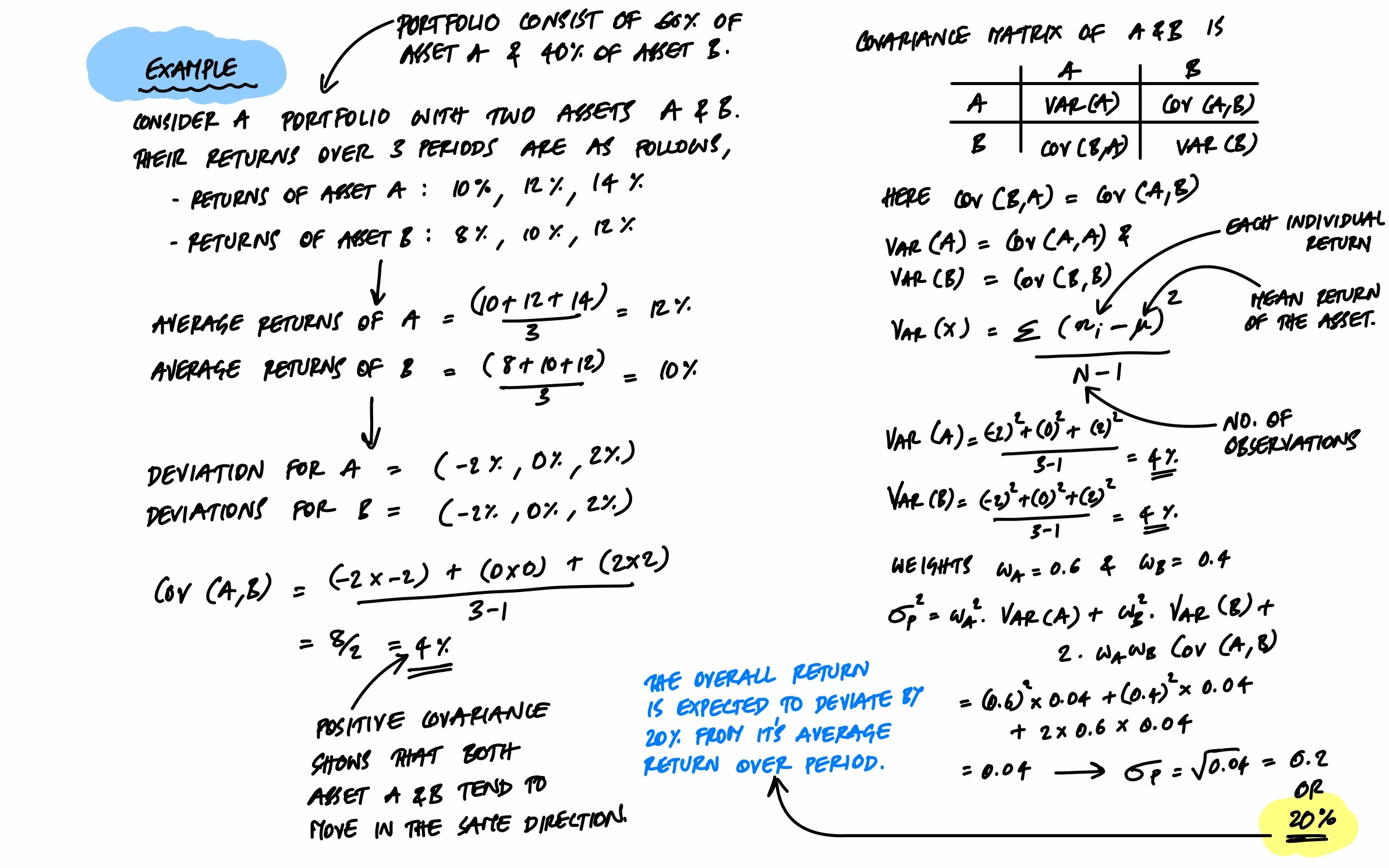
The expected return of a portfolio is simply the weighted average of the returns of its individual assets. If you put 60% in equities (expected return 10%) and 40% in bonds (expected return 5%), your portfolio's expected return is 0.6 × 10% + 0.4 × 5% = 8%.

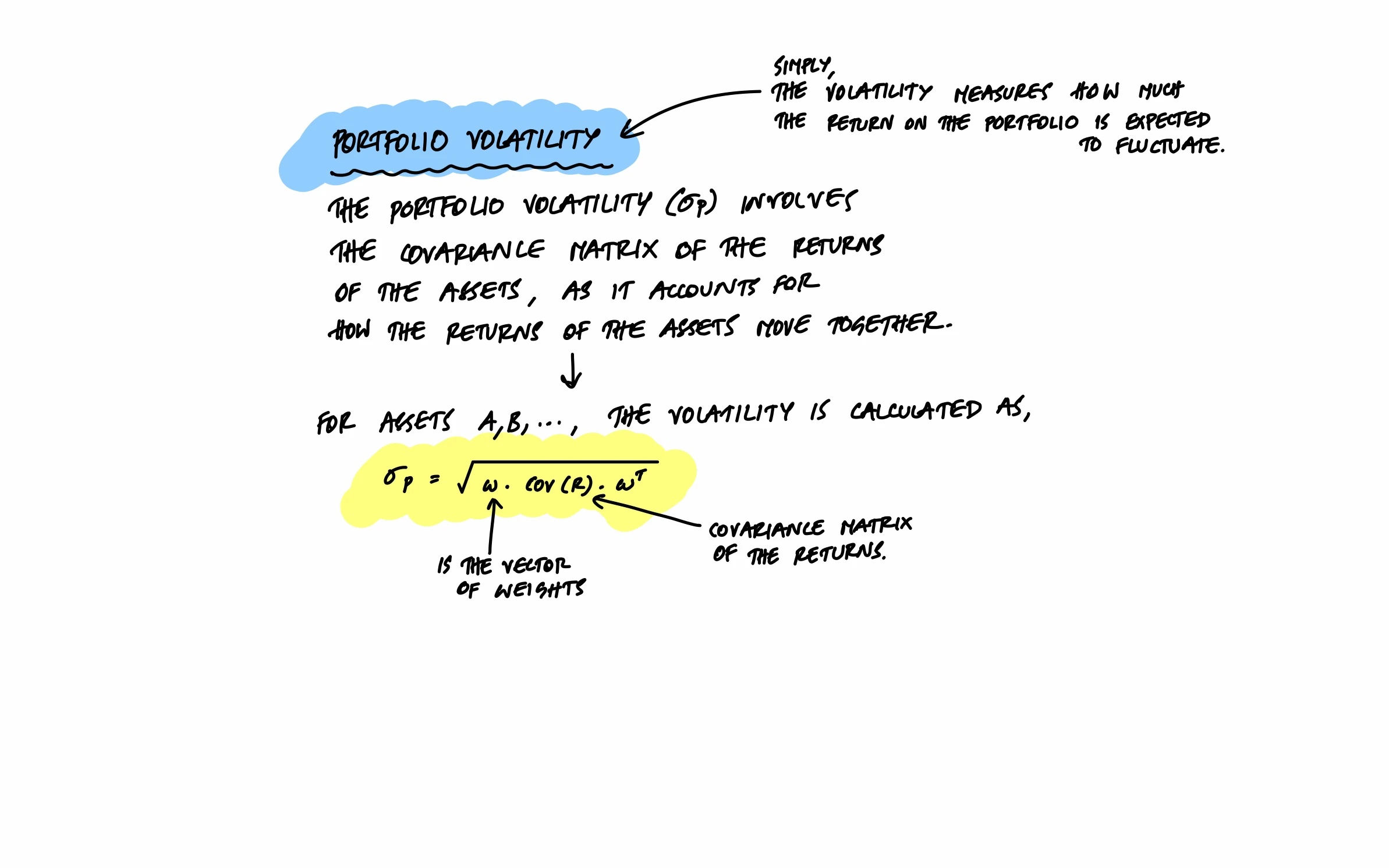
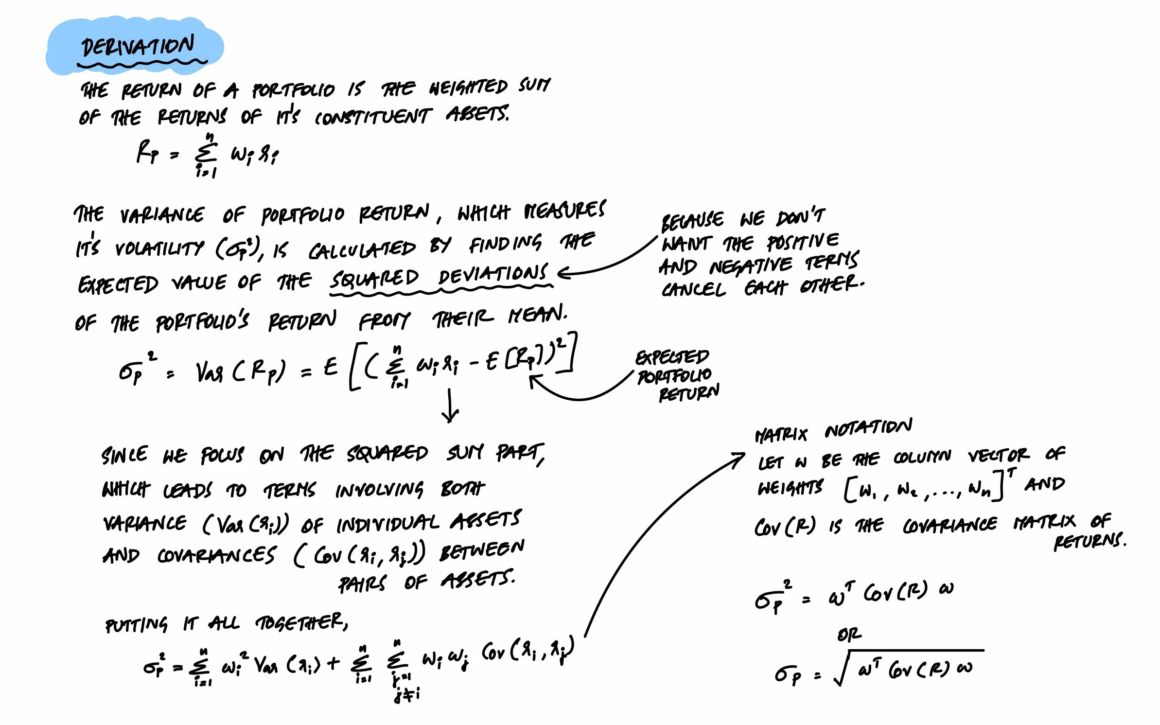
Portfolio Volatility

Here's where it gets interesting. The volatility (risk) of a portfolio is not simply the weighted average of individual asset volatilities. It also depends on the covariance between assets - how their returns move together. This is the mathematical basis for diversification: if assets don't move in lockstep, combining them reduces overall portfolio risk.

Correlation and Diversification

Correlation coefficients measure how two assets move relative to each other. They range from -1 to 1:

• +1: Perfect positive correlation - assets always move together. No diversification benefit.
• 0: No correlation - assets move independently. Good diversification.
• -1: Perfect negative correlation - assets move in opposite directions. Maximum diversification benefit.

Using hypothetical 5-year returns for three asset classes, the correlations work out to:

• Equities & Bonds: 0.55 - moderate positive correlation. They tend to move somewhat together, but not perfectly.
• Equities & Gold: -0.06 - nearly independent. Gold can act as a hedge when equities are volatile.
• Bonds & Gold: -0.65 - moderate negative correlation. Gold tends to rise when bond yields fall, making them effective diversification partners.

By combining assets with low or negative correlations, you can build a portfolio where the overall volatility is lower than the volatility of any single asset in it. This is the power of diversification, expressed mathematically.

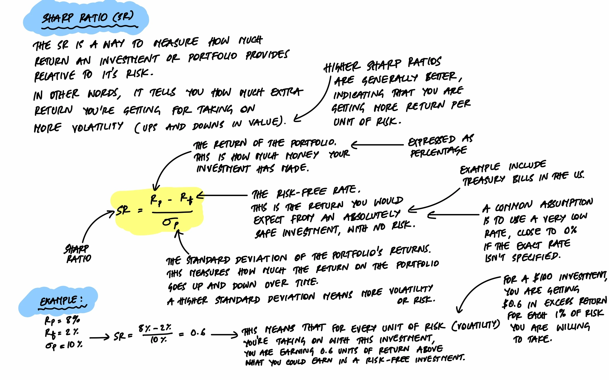
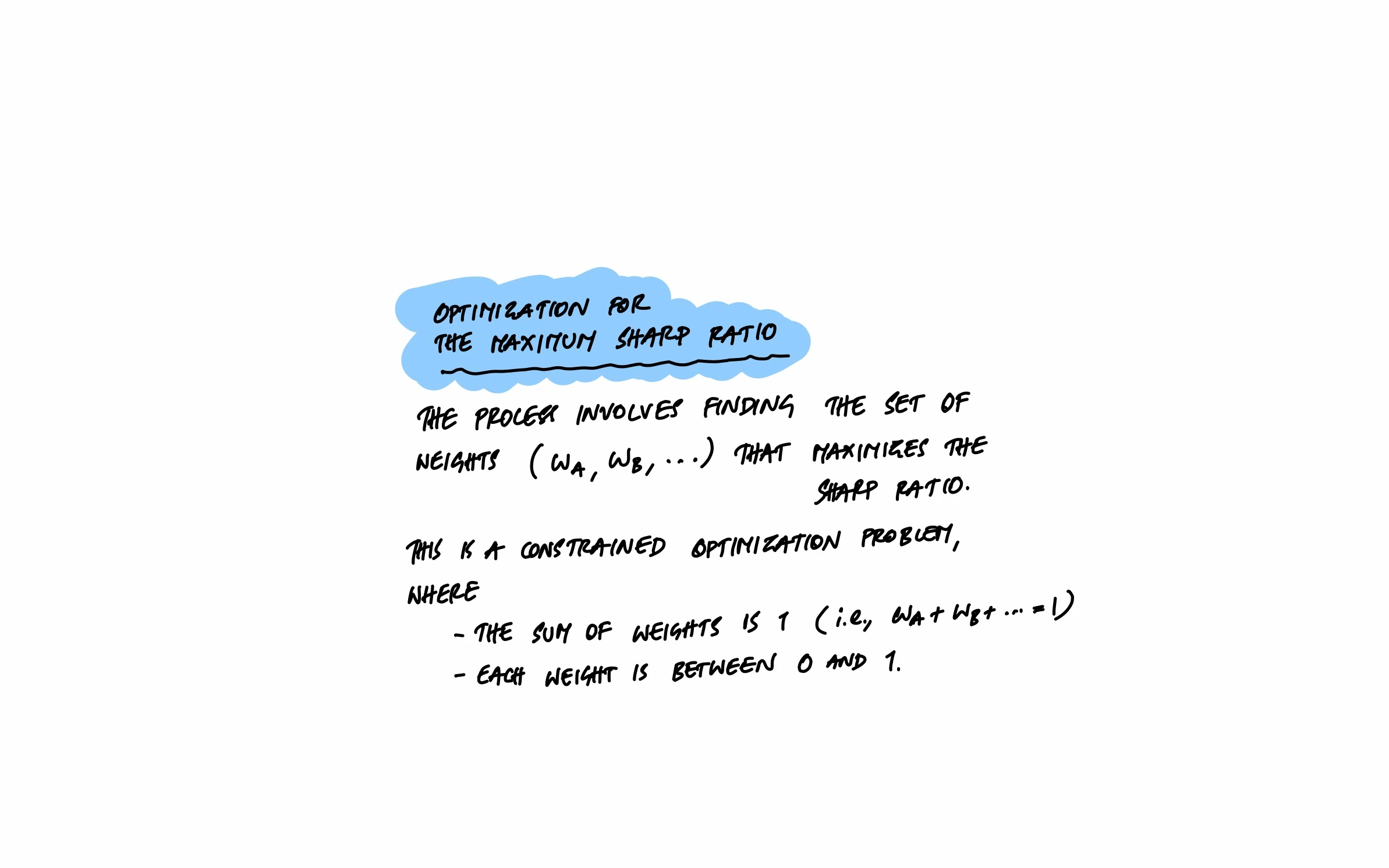
The Sharpe Ratio

To compare portfolios, we need a way to measure risk-adjusted return - how much return you're getting per unit of risk. The Sharpe Ratio does exactly this: it takes the portfolio's return, subtracts the risk-free rate (what you'd earn from a completely safe investment like treasury bills), and divides by the portfolio's volatility. A higher Sharpe Ratio means you're being better compensated for the risk you're taking.

The Efficient Frontier

Now we can put it all together. Given three asset classes (equities, bonds, and gold) with known returns, volatilities, and correlations, we can generate thousands of random portfolio combinations and plot them by expected return vs. volatility. The result is the Efficient Frontier.

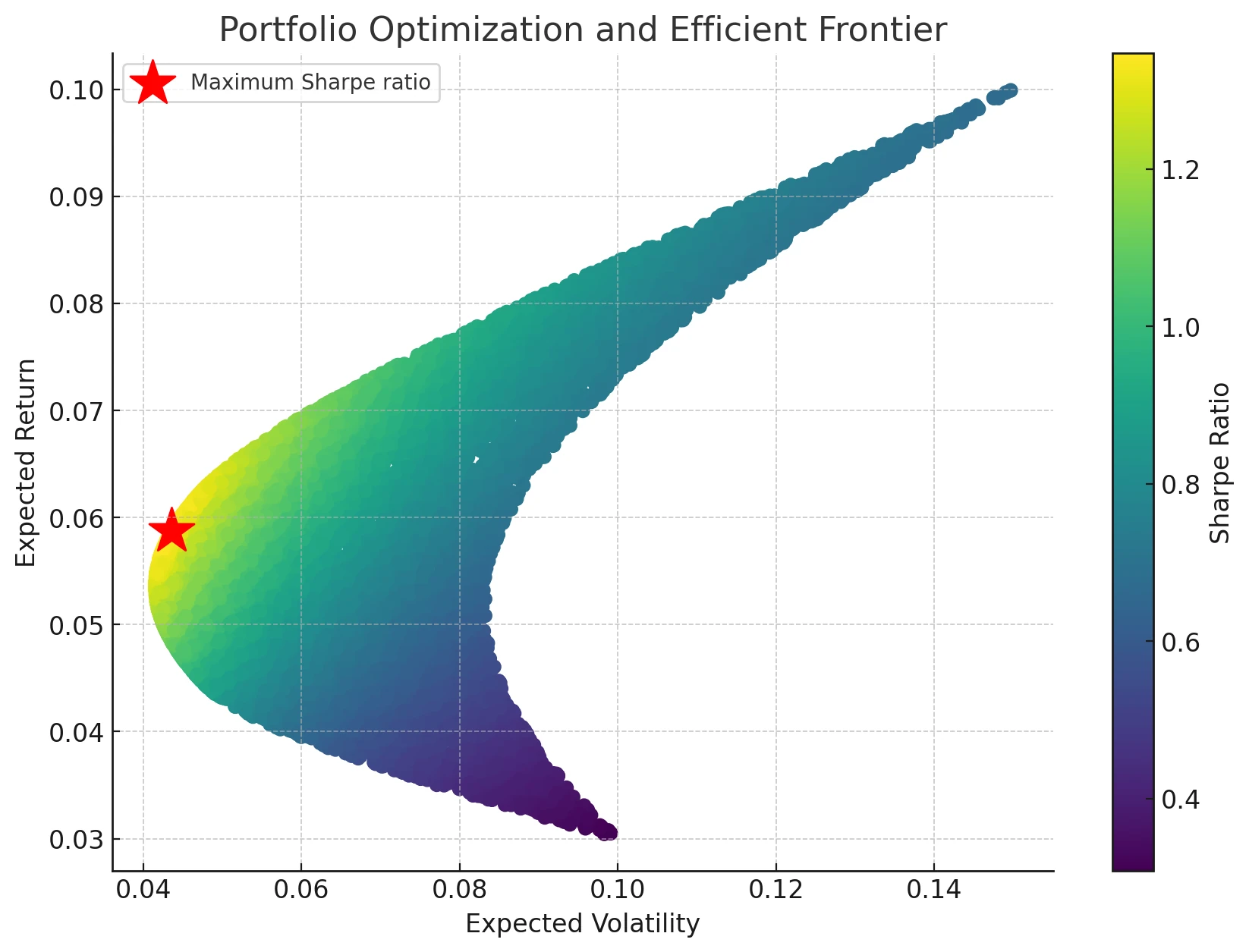
Each point on this plot is a different portfolio. The color represents the Sharpe Ratio - warmer colors indicate better risk-adjusted returns. The star marks the portfolio with the maximum Sharpe Ratio: the optimal balance of risk and return.

For this example, the optimal portfolio has:

• Expected return: ~5.87% per annum
• Expected volatility: ~4.36% per annum
• Sharpe Ratio: ~1.35
• Allocation: ~19.5% equities, ~75.2% bonds, ~5.3% gold

This might surprise you - the "optimal" portfolio is heavily weighted toward bonds, not equities. That's because the optimization maximizes risk-adjusted return, not absolute return. The small allocation to equities captures some growth, while bonds provide stability, and gold adds a diversification benefit due to its low correlation with the other assets. The Efficient Frontier gives you the framework to choose any point along the curve based on how much risk you're willing to accept.

Keeping It on Track: Rebalancing

Building the right portfolio is only half the job. Over time, market movements will push your actual allocation away from your target. If equities have a strong year, they'll grow to represent a larger share of your portfolio than intended - meaning you're now taking more risk than you planned for.

How Rebalancing Works

Say your target allocation is 50% equities, 30% bonds, 20% gold, and your portfolio has grown to ₹10,00,000. After a year of market movements, the actual allocation has drifted to 60% equities, 25% bonds, 15% gold. Here's the math:

• Equities: Current ₹6,00,000 → Target ₹5,00,000. Sell ₹1,00,000.
• Bonds: Current ₹2,50,000 → Target ₹3,00,000. Buy ₹50,000.
• Gold: Current ₹1,50,000 → Target ₹2,00,000. Buy ₹50,000.

You're selling what's gone up (equities) and buying what's lagged (bonds, gold). This is systematically buying low and selling high - which is exactly what good investing is supposed to look like.

Does Rebalancing Actually Help?

To test this, we can simulate a 60/40 equities-bonds portfolio over 10 years under three market conditions - bullish, bearish, and volatile - comparing rebalanced vs. unrebalanced performance:

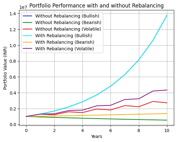
The results are telling:

• Bullish markets: The unrebalanced portfolio ends up slightly higher, because equities keep growing and take over a larger share. But it also carries significantly more risk.
• Bearish markets: The rebalanced portfolio outperforms, because it systematically reduced equity exposure as markets fell and maintained the stabilizing effect of bonds.
• Volatile markets: Rebalancing smooths out the ups and downs, reducing the emotional stress of watching your portfolio swing wildly.

Rebalancing isn't about maximizing absolute returns - it's about maintaining the risk level you chose and staying disciplined through market cycles. Over long horizons, this discipline tends to produce better risk-adjusted outcomes.

Key Takeaway

Investment planning doesn't have to be guesswork. The tools exist to answer the hard questions quantitatively: compound interest tells you how your money grows, Monte Carlo simulations show you the range of possible outcomes, Modern Portfolio Theory helps you find the optimal mix of assets, and rebalancing keeps your plan on track over time.

None of this requires expensive advisors or proprietary software. The formulas are well-established, the data is publicly available, and tools like Python (with pandas, NumPy, and Matplotlib) or even a well-structured spreadsheet can run these calculations. What it does require is taking the time to define your goals, understand your risk tolerance, and let the math guide your decisions instead of emotions.

Start simple: calculate your retirement number using compound interest. Run a basic Monte Carlo simulation to see the range of outcomes. Check whether your current portfolio allocation matches your risk profile. Each step builds on the last, and each one gives you more confidence that your investment plan is grounded in something real.