


A Quantitative Approach to Personalized Investment Planning
- Visakh Unni

- Jan 29, 2025
- 14 min read

Defining Financial Goals and Investment Horizon
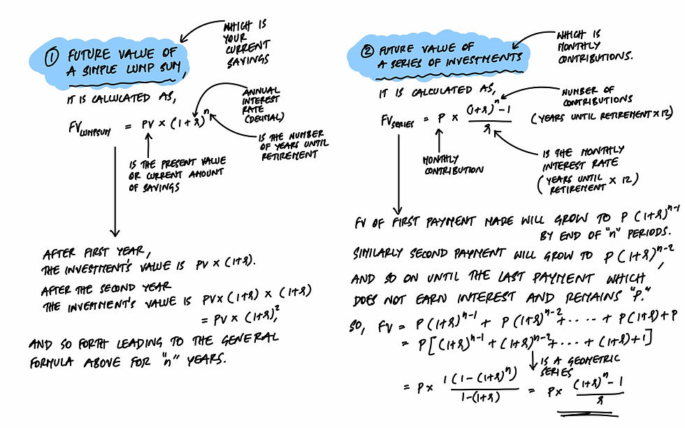
Time Value of Money (TVM) Calculations: To estimate the future value of current savings and investments or the amount needed to save to meet a financial goal (retirement planning, buying a house, funding education). The formula involves calculating compound interest over time.
Example: Suppose you are planning to save for your retirement, which is 25 years away. You currently have ₹500,000 in savings, and you plan to contribute ₹10,000 monthly towards your retirement fund. Assuming an average annual return of 7% (which is a realistic figure for a diversified investment portfolio in India), let's calculate the future value of your retirement fund using the formula for the future value of a series of investments (annuity) combined with the future value of a single lump sum.
The future value FV of an investment is given by two parts in this scenario:
Let's calculate both parts to find the total future value of your retirement fund.
Based on the calculations:
The future value of your current savings (₹500,000) alone, compounded annually at a 7% rate of return over 25 years, would be approximately ₹2,713,716.
The future value of your monthly contributions (₹10,000 per month) at the same rate, compounded monthly over the same period, would be approximately ₹8,100,717.
Combining both, the total future value of your retirement fund would be approximately ₹10,814,433.
This means, under the given conditions, you could expect to have around ₹10.8 million in your retirement fund in 25 years. This calculation illustrates the power of compound interest and regular investing over time
Which Is Better?
Market Upturns: The lump sum investment generally performs better in markets that trend upwards over the long term, as the initial larger amount has more time to compound.
Volatility and Downturns: The series of investments can sometimes outperform in volatile or downtrending markets, as it allows for dollar-cost averaging, potentially buying more shares when prices are low.
So use a combination of both.
Simulations:
Monte Carlo Simulations: To project various scenarios for how an investment might grow over time, given a range of variables such as rate of return, inflation, and contributions. These simulations can help estimate the probability of reaching financial goals within different time horizons (short-term, medium-term, long-term).
Why Use Monte Carlo Simulations?
Monte Carlo simulations are particularly valuable in situations where:
The problem involves a significant level of uncertainty and variability.
Analytical or exact solutions are difficult or impossible to obtain due to the complexity of the model.
You want to assess the risk and probabilities of different outcomes to make informed decisions.
Basic Concept: The core idea of Monte Carlo simulations is to use randomness to solve problems that might be deterministic in principle. These simulations draw upon the law of large numbers, implying that as the number of trials increases, the average result will converge to the expected value.
Financial Application Example
In finance, Monte Carlo simulations are often used to estimate the future value of an investment portfolio over time, considering the variability and uncertainty in returns. Here's a breakdown of how it's applied:
Define Probability Distributions: For each variable that influences the outcome (e.g., annual return rates of different assets), define a probability distribution based on historical data or future expectations. This includes the mean (average return) and standard deviation (volatility) of returns.
Random Sampling: Randomly sample values from the probability distributions defined for each variable. This simulates one possible outcome based on the expected variability of each variable.
Compute Each Trial: Use the sampled values to compute the result of each trial. For a portfolio simulation, this could involve calculating the portfolio's total value each year over the investment horizon, given the randomly sampled return rates for each year.
Repeat: Repeat steps 2 and 3 many times (e.g., 1,000 or 10,000 trials) to generate a wide range of possible outcomes.
Analyze Results: Aggregate the results of all trials to analyze the statistical properties of the portfolio's future value. This can include calculating the mean, median, variance, and plotting the distribution of outcomes to visualize the probability of different results.
Example: Consider an investment scenario similar to the previous example but with a twist: instead of assuming a constant rate of return, we'll simulate various rates of return to reflect the uncertainty and volatility of real-world investments. We'll also incorporate annual contributions to the investment.
Scenario Parameters:
Initial Investment (Present Value, PV): ₹500,000
Annual Contribution: ₹120,000 (₹10,000 monthly)
Investment Horizon: 25 years
Expected Annual Return Rate: 7% (average)
Standard Deviation of Annual Return Rate: 3% (to introduce variability)
Number of Simulations: 1,000 (to capture a wide range of potential outcomes)
We'll simulate each year's rate of return as a random variable following a normal distribution centered around the expected annual return rate with a standard deviation that captures the variability in returns. The total investment value at the end of each year will consider both the return on the existing investment and the new contribution for that year.
The outcome will give us a distribution of possible future values for the investment, from which we can derive probabilities for reaching specific financial goals.
Let's perform the simulation and generate figures to illustrate the distribution of potential outcomes.

The Monte Carlo simulation of your investment growth over 25 years, with 1,000 different scenarios, is illustrated above. Each blue line represents a potential path your investment could take, given the variability in annual returns. The red line shows the average outcome across all simulations.
This approach provides a visual and quantitative method to assess the range of possible future values of your investment, considering the volatility and uncertainty inherent in financial markets. It helps in understanding the likelihood of achieving specific financial goals within your investment horizon.
The wide spread of outcomes highlights the risk and potential reward of investing. For individual investors, such simulations underscore the importance of maintaining a diversified portfolio and a long-term perspective, especially in markets like India, where economic growth prospects can lead to significant investment opportunities amidst volatility.
Understanding Your Risk Tolerance
Risk Assessment Questionnaires: Standardized questionnaires can provide a quantitative measure of risk tolerance based on responses to various scenarios and preferences.
Example: Risk assessment questionnaires are pivotal in financial planning, helping to align investment strategies with an individual's risk tolerance. Below is a simplified example of how such a questionnaire might look, along with a method to score responses and interpret the results to quantify risk tolerance.
Example Risk Assessment Questionnaire
For each question, choose the option that best describes your investment preference or reaction. Each answer has a score associated with it. Your total score will help determine your risk tolerance level.
Investment Goal and Time Horizon
A. Preservation of capital with a time horizon of less than 2 years. (Score: 1)
B. Income with a moderate growth expectation and a time horizon of 3-5 years. (Score: 2)
C. Growth as the main goal with a time horizon of more than 6 years. (Score: 3)
Experience with Investments
A. None. (Score: 1)
B. Limited; mostly traditional investments (e.g., fixed deposits, bonds). (Score: 2)
C. Experienced; includes stocks, mutual funds, and other securities. (Score: 3)
Reaction to Market Downturns
A. Would sell investments to minimize losses. (Score: 1)
B. Would hold investments and wait for markets to recover. (Score: 2)
C. Would see it as a buying opportunity to invest more. (Score: 3)
Expected Rate of Return
A. Up to 5% per annum, with very low risk. (Score: 1)
B. Between 5% to 10% per annum, with moderate risk. (Score: 2)
C. More than 10% per annum, willing to accept high volatility. (Score: 3)
Income Requirement
A. Need to rely on my investments for current income. (Score: 1)
B. Don't need immediate income but prefer investments that generate some income. (Score: 2)
C. Do not need any income from investments and prefer reinvesting income to grow my portfolio. (Score: 3)
Calculating Risk Tolerance
After answering all questions, sum up the scores. The total score will determine the investor's risk tolerance:
5-8 Points: Low Risk Tolerance. Prefers investments with minimal risk, even if it means lower returns. Suitable for conservative investment vehicles like fixed deposits, bonds, or stable value funds.
9-12 Points: Moderate Risk Tolerance. Comfortable with a balanced mix of investments, including equities and fixed income. Suitable for balanced mutual funds or hybrid funds.
13-15 Points: High Risk Tolerance. Primarily seeks capital growth and is willing to accept significant fluctuations in investment value. Suitable for diversified equity portfolios, high-growth mutual funds, or ETFs.
This simplified questionnaire and scoring system provides a foundational approach to understanding an investor's risk profile. It's essential to remember that risk tolerance is just one aspect of financial planning. Goals, financial situation, and market conditions should also be considered when crafting an investment strategy.
Simulations:
Portfolio Volatility Simulations: Using historical market data to simulate the volatility of a hypothetical portfolio, helping to visually understand potential ups and downs in investment value.
Example: To demonstrate portfolio volatility simulations, we'll use a simplified approach, focusing on a hypothetical portfolio composed of two main asset classes often found in diversified portfolios:
Equities (Stocks)
Fixed Income (Bonds)
For this example, let's assume the following asset allocation, which reflects a moderate risk profile:
60% Equities
40% Bonds
Historical Annual Returns
We'll use hypothetical historical annual returns to simulate portfolio volatility. For simplicity, let's assume the following average returns and standard deviations (which are somewhat reflective of long-term market behavior):
Equities:
Average Return: 10%
Standard Deviation: 15%
Bonds:
Average Return: 5%
Standard Deviation: 5%
Simulation Parameters
Investment Horizon: 20 years
Number of Simulations: 1000
We'll simulate the portfolio's annual returns based on the asset allocation, using the average returns and standard deviations for equities and bonds. The total portfolio return for each year will be a weighted average of the returns from equities and bonds, adjusted for their respective allocations in the portfolio.
The goal is to illustrate the range of potential outcomes for the portfolio's value over time, highlighting the volatility and the risk/return trade-off.
Let's perform the simulation and generate a figure showing the distribution of portfolio values over the 20-year horizon.

The figure illustrates the simulated values of a hypothetical portfolio over 20 years, under 1,000 different scenarios, reflecting the combined volatility of equities and bonds based on historical performance characteristics. Each light blue line represents a possible trajectory for the portfolio's value, relative to the initial investment, highlighting the variability in potential outcomes due to market volatility.
The red line indicates the median outcome across all simulations, offering a sense of the most typical path the portfolio might take, considering the mix of assets and their historical returns and volatilities.
Why Median is Taken Instead of Average
The median is the middle value in a dataset when it has been arranged in ascending or descending order. It's robust to outliers, meaning it's not affected by extremely high or low values. In the context of this simulation, using the median provides a view of the "typical" outcome that is not skewed by extreme results. This can give a more representative idea of the expected outcome, especially in scenarios where the distribution of outcomes is not symmetric or has outliers.
This simulation underscores the importance of understanding portfolio volatility and the range of possible outcomes, especially for long-term investors. It visually demonstrates the ups and downs an investor might experience, reinforcing the concept that while equities may introduce more volatility into a portfolio, the combination with bonds can provide a balance, potentially smoothing out returns over time in a diversified portfolio.
Asset Allocation
Efficient Frontier and Modern Portfolio Theory (MPT): To determine the optimal mix of assets that offers the best return for a given level of risk. This involves solving an optimization problem to find the asset allocation that maximizes the portfolio's expected return for a given risk level.
Example: To illustrate the Efficient Frontier and Modern Portfolio Theory (MPT), let's consider a simplified example with three asset classes:
Equities (Stocks)
Bonds
Gold
We will calculate the expected returns, volatilities (standard deviations), and correlations among these asset classes. Then, we'll use this data to find the optimal asset allocations for various levels of risk, showcasing the Efficient Frontier.
Hypothetical Data
Expected Annual Returns:
Equities: 10%
Bonds: 5%
Gold: 3%
Annual Volatility (Standard Deviation):
Equities: 15%
Bonds: 5%
Gold: 10%
Correlation Matrix (for simplicity, let's assume):
Equities & Bonds: -0.2
Equities & Gold: 0
Bonds & Gold: 0.1
Objective
The objective is to minimize the portfolio variance for a given expected return, or equivalently, to maximize the expected return for a given level of risk. This involves calculating the weights of each asset class in the portfolio that lead to the optimal risk-return trade-off.
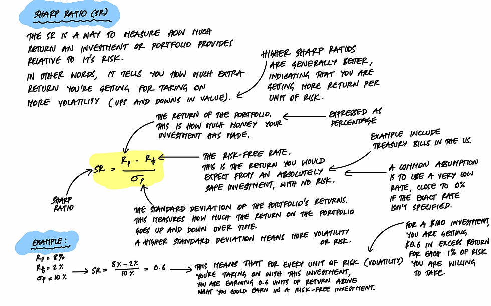
Sharp Ratio
Steps
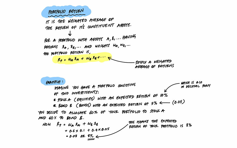
Calculate the Portfolio Expected Return:
This is the weighted average of the expected returns of the asset classes.
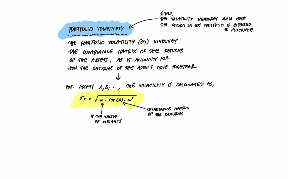
Calculate the Portfolio Variance:
This considers the variances of each asset class and their correlations.


Optimization:
Use these calculations to generate a set of portfolios that represent the Efficient Frontier.
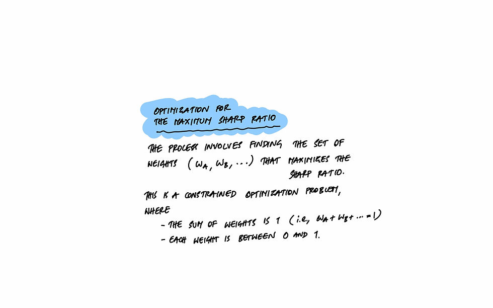
For simplicity, let's create a series of portfolios with varying levels of risk by adjusting the weights of the asset classes, and then identify the Efficient Frontier from these portfolios.
Let's proceed with the calculations and plot the Efficient Frontier.

The corrected visualization above shows the results of our portfolio optimization analysis, including the Efficient Frontier in the context of Modern Portfolio Theory (MPT). Each point represents a different portfolio composition with varying allocations of equities, bonds, and gold.
The color gradient represents the Sharpe ratio of each portfolio, with warmer colors indicating higher Sharpe ratios, signifying a better risk-adjusted return.
The star marker highlights the portfolio with the maximum Sharpe ratio, representing the optimal risk-return balance according to the Sharpe ratio criterion.
This plot demonstrates how investors can use MPT and the Efficient Frontier to make informed decisions about asset allocation. By choosing a point on the frontier, investors can aim for the highest possible return for a given level of risk. The portfolio marked by the star suggests an optimal allocation that balances expected return and risk in an efficient manner, maximizing the Sharpe ratio.
Expected Return: Approximately 5.87% per annum
Expected Volatility: Approximately 4.36% per annum
Sharpe Ratio: Approximately 1.35, indicating a favorable risk-adjusted return
Optimal Asset Allocation:
Equities: Approximately 19.51%
Bonds: Approximately 75.23%
Gold: Approximately 5.26%
Simulations:
Historical Backtesting: To test how a particular asset allocation would have performed in the past, helping investors understand potential returns and losses.
Diversification
Correlation Coefficients: To analyze the degree to which different assets move in relation to one another, with the aim of selecting assets that do not perfectly correlate, reducing overall portfolio risk.
Example: To demonstrate how correlation coefficients work and how they can be used to reduce overall portfolio risk, let's use a simplified example with three asset classes: Equities, Bonds, and Gold. We'll calculate the correlation coefficients among these asset classes based on hypothetical annual return data. Correlation coefficients range from -1 to 1, where:
1 indicates a perfect positive correlation (assets move in the same direction),
-1 indicates a perfect negative correlation (assets move in opposite directions),
0 indicates no correlation (assets move independently of each other).
Hypothetical Annual Returns
Imagine we have 5 years of annual returns for each asset class:
Equities Returns (%): 10, -5, 15, 7, 12
Bonds Returns (%): 5, 3, 4, 5, 4
Gold Returns (%): -2, 1, 0, -1, 3
Objective
Calculate the correlation coefficients among these asset classes to identify how they move in relation to each other, aiming to construct a diversified portfolio that minimizes risk.
Let's proceed with the calculations.
The correlation coefficients among Equities, Bonds, and Gold, based on the hypothetical annual returns, are as follows:
Equities & Bonds: 0.55
Equities & Gold: -0.06
Bonds & Gold: -0.65
Interpretation:
Equities & Bonds have a moderate positive correlation of 0.55, suggesting that they tend to move somewhat in the same direction but not perfectly. Including both in a portfolio can provide some diversification benefits.
Equities & Gold have a very low negative correlation of -0.06, indicating they move almost independently of each other. This provides a good diversification opportunity, as gold can act as a hedge or safe haven when equities are volatile.
Bonds & Gold have a moderate negative correlation of -0.65, meaning they tend to move in opposite directions. This is beneficial for diversification, as gold's price often increases when bond yields (which move inversely to bond prices) are falling or when investors are seeking safety away from traditional fixed-income investments.
By selecting assets with low or negative correlations, investors can construct a portfolio that may lower overall risk through diversification. In this example, including all three asset classes—Equities, Bonds, and Gold—could potentially reduce portfolio volatility, as their returns do not move perfectly in tandem.
Choosing the Right Investment Vehicles
Simulations:
Comparison Analysis: Using data analysis tools to compare historical performance, fees, and risk levels of different investment vehicles like mutual funds, ETFs, and bonds.
Review and Rebalance
Rebalancing Algorithms: To determine when and how much to buy or sell from each asset category to return the portfolio to its target asset allocation.
Example: To illustrate how rebalancing algorithms work, let's consider a simplified portfolio that consists of three asset categories: Equities, Bonds, and Gold. The initial target asset allocation for a moderate risk profile might be:
Equities: 50%
Bonds: 30%
Gold: 20%
Suppose over time, due to market movements, the actual portfolio allocation has drifted to:
Equities: 60%
Bonds: 25%
Gold: 15%
And let's assume the total portfolio value has grown to ₹1,000,000.
The goal of rebalancing is to adjust the investments back to the target allocation. We'll calculate how much of each asset category needs to be bought or sold to achieve this.
Steps for Rebalancing
Calculate the target value for each asset category based on the target allocation percentages and the total portfolio value.
Determine the current value of each asset category based on the drifted allocation percentages and the total portfolio value.
Calculate the difference between the current value and the target value for each asset category. A positive difference indicates a need to buy more of the asset, while a negative difference indicates a need to sell.
Let's perform these calculations.
Based on the target and current allocations, here are the calculated values and necessary adjustments:
Target Values:
Equities: ₹500,000
Bonds: ₹300,000
Gold: ₹200,000
Current Values (After Drift):
Equities: ₹600,000
Bonds: ₹250,000
Gold: ₹150,000
Rebalancing Actions (To Return to Target Allocation):
Equities: Sell ₹100,000 (to reduce from ₹600,000 to ₹500,000)
Bonds: Buy ₹50,000 (to increase from ₹250,000 to ₹300,000)
Gold: Buy ₹50,000 (to increase from ₹150,000 to ₹200,000)
These rebalancing actions are necessary to adjust the portfolio back to its intended target allocation of 50% equities, 30% bonds, and 20% gold, aligning the investments with the investor's risk tolerance and investment strategy. This process of buying or selling assets to maintain the desired asset allocation helps manage risk and can contribute to achieving long-term investment goals.
Simulations:
Rebalancing Impact Simulations: To assess the potential impact of rebalancing on portfolio performance under various market conditions.
Example: To assess the impact of rebalancing on portfolio performance under various market conditions, we'll simulate a portfolio's performance over a 10-year period. We'll compare two scenarios:
Without Rebalancing: The portfolio's asset allocation drifts according to market returns, with no adjustments.
With Rebalancing: The portfolio is rebalanced annually back to its target asset allocation.
Portfolio and Market Conditions:
Initial Asset Allocation: 60% Equities, 40% Bonds
Target Allocation for Rebalancing: Same as initial
Initial Portfolio Value: ₹1,000,000
Annual Return Rates (Hypothetical):
Equities: Bullish Market: 12%, Bearish Market: -8%, Volatile Market: 12%/-8% alternating
Bonds: Steady Return of 5% across all market conditions
Simulation Steps:
Calculate annual returns for both assets under each market condition.
Apply these returns to the portfolio to simulate performance over 10 years, with and without rebalancing.
Compare the final portfolio values and visualize the results.
Let's perform this simulation and generate the graph.
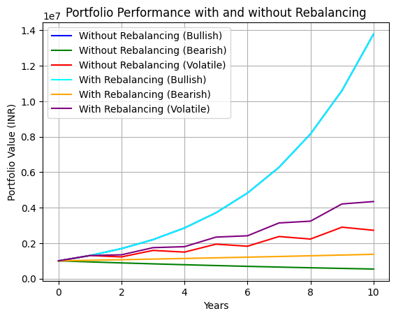
The graph illustrates the performance of a portfolio over 10 years under different market conditions: bullish, bearish, and volatile, both with and without annual rebalancing back to the target asset allocation of 60% equities and 40% bonds.
Bullish Market Scenario: The portfolio without rebalancing ends up with a higher value due to the higher returns from equities dominating the portfolio over time. However, the rebalanced portfolio, while slightly lower in value, likely experienced less volatility due to maintaining the target allocation.
Bearish Market Scenario: The rebalanced portfolio outperforms the one without rebalancing, as rebalancing helps to reduce the impact of the declining equity market by ensuring that bonds, with their steadier returns, make up the intended portion of the portfolio.
Volatile Market Scenario: The rebalanced portfolio smoothens out the highs and lows experienced by the portfolio without rebalancing, illustrating the benefit of rebalancing in reducing volatility.
This simulation highlights the impact of rebalancing on portfolio performance, showing how maintaining a target asset allocation can help manage risk and potentially improve the risk-adjusted returns of a portfolio across various market conditions.
Staying Informed and Flexible
While this step is more qualitative, staying informed through financial news, market trends, and economic indicators can be supported by tools like financial news aggregators, market analysis software, and investment platforms that offer alerts and insights.
Tools and Frameworks
For executing these models and simulations, there are various financial planning software and platforms, spreadsheets (like Excel with its Solver function for optimization problems), and programming languages like Python, which has libraries (pandas, NumPy, Matplotlib, SciPy) for data analysis, statistical modeling, and visualization.
Implementing these models and simulations requires a blend of financial knowledge, access to historical and real-time data, and proficiency in using financial planning tools or programming languages.
Comments